Intelligent Systems · Project P4 · November 2026

Learned delivery routing

A dispatcher has twenty deliveries with time windows and three vans. A neural network learns how long New York trips take at each hour, a constraint solver gives each order a van, and A* finds each van's best stop order. When a route runs late, the system learns a new rule and plans again.

Slides Project dossier Report

P4The system

How the three parts fit

Each part answers one question: how long a trip takes, which van takes an order, and in what order a van drives.

4Learn

Neural network

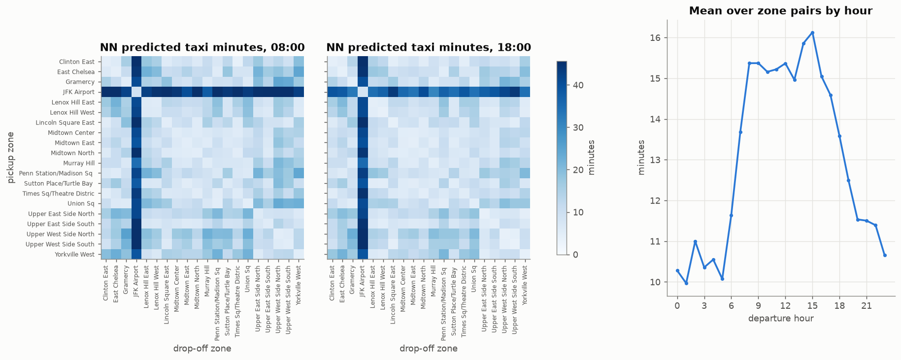
A numpy MLP predicts trip minutes from pickup zone, drop-off zone, hour, weekday and typical distance. Output: a 24 × 20 × 20 hourly time matrix.

→

6Assign

Constraint solver

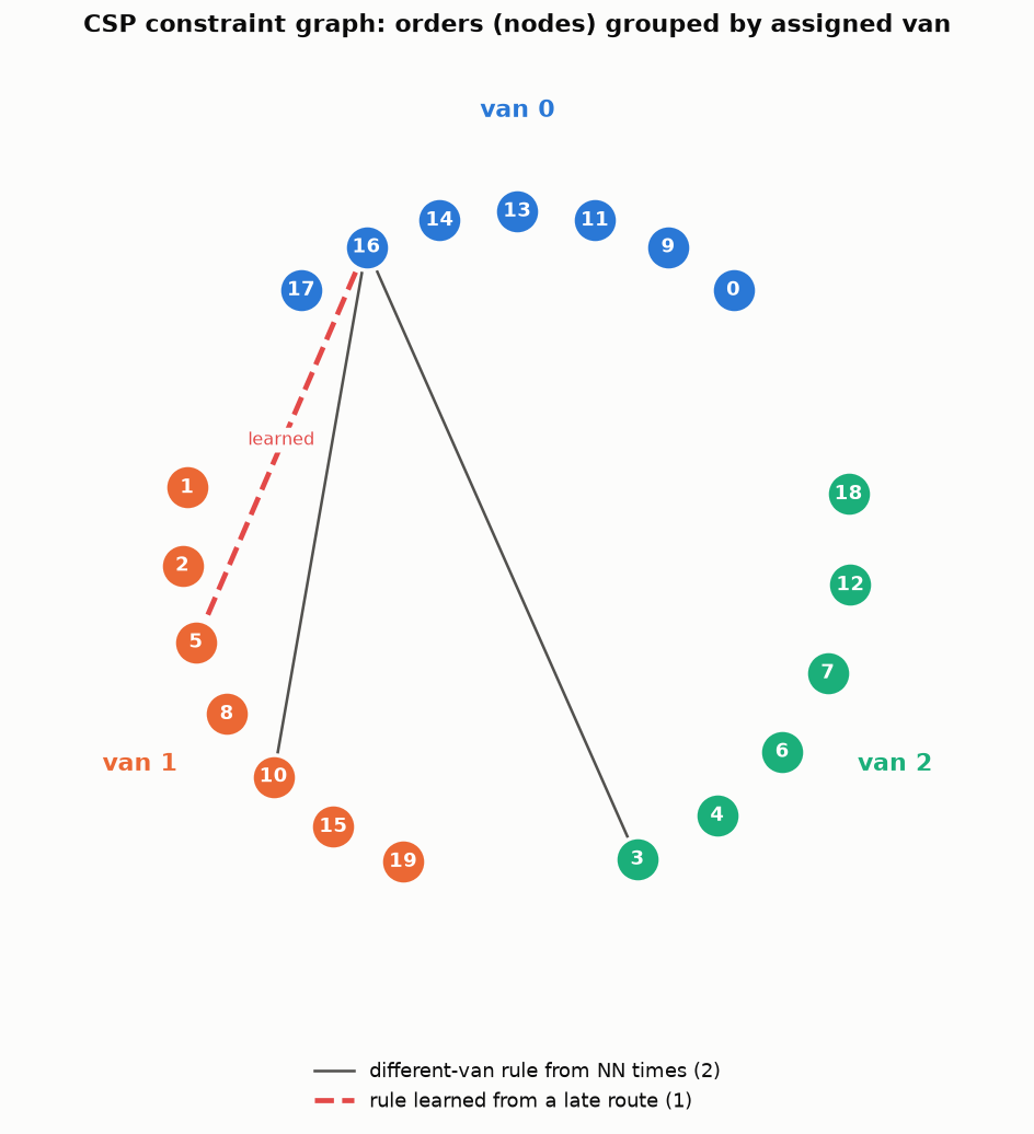
Variable = van per order. Rules: the window is reachable from the depot, capacity, at most 10 stops, and "different van" pairs derived from the NN times. Backtracking, Forward Checking and AC-3 are switchable.

→

5Order

A* search

State = (stop, visited set, clock). Cost = travel plus waiting. An admissible time-dependent heuristic; UCS and Greedy as baselines.

Feedback. if a van's best route is still late, the first late pair becomes a new "different van" rule and the CSP runs again (up to 5 loops). If nothing works, the system reports which orders are unserviceable and why, and tries widening windows in 15-minute steps.

2Code and data line · stop 2 in the dossier

Data

NYC Taxi & Limousine Commission trip records, January 2022. From 2.46 M yellow-taxi trips we keep weekdays, durations of 1 to 120 minutes and the 20 busiest zones (19 in Manhattan plus JFK), about 300 k trips. The split is by day: three weeks to train, the last week to test.

Orders, time windows, demands and van capacities are generated by a seeded generator (15, 20 and 30 orders × 10 seeds). Taxi times only approximate van times, so we apply a documented van factor of 1.2.

Step	Trips
Yellow taxi, Jan 2022	2.46 M
Weekdays, 1–120 min, valid zones	filtered
Both ends in the top-20 zones	≈ 300 k
Test set (last week)	93,592

4Models line · stop 4 in the dossier

Travel-time model

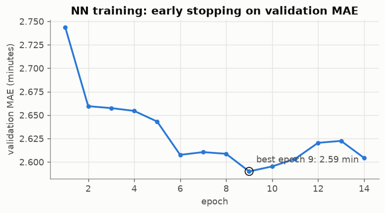
A hand-written numpy MLP: zone one-hots (acting as embeddings), hour and weekday encodings and the pair distance, trained with Adam, Huber loss and early stopping. Compared against three baselines on the same held-out week.

Model	MAE (min)	RMSE	Bias
NN (MLP)	3.23	5.44	−1.87
Historical average (pair, hour)	3.24	5.42	−1.61
Distance-linear	4.14	6.40	−1.62
Global mean	5.45	8.88	−1.31

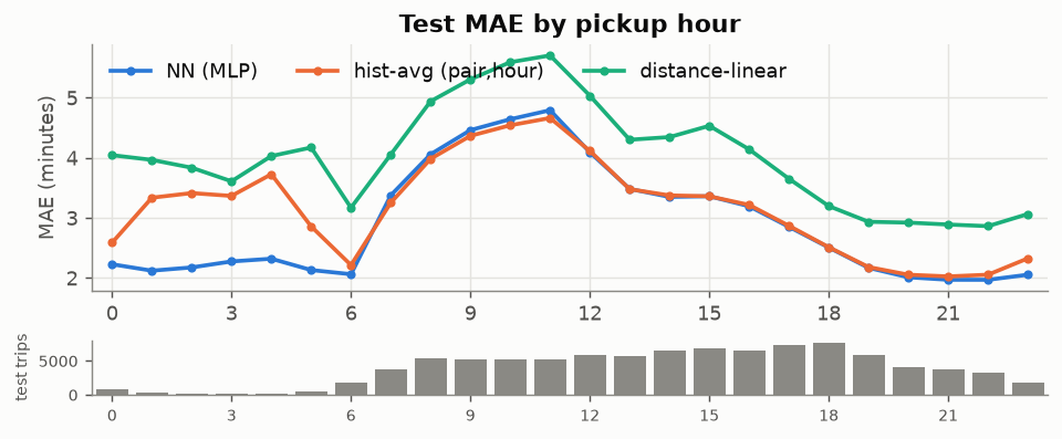
Overall, the NN is tied with the historical lookup table. Its advantage shows on rare (pair, hour) cells with fewer than 3 training trips: MAE 3.25 vs 4.69. Every model under-predicts the slower test week by about 1.7 minutes.

Training and validation loss per epoch — Learning curve with early stopping.

Mean absolute error by hour for each model — Error by hour of day, all models.

Predicted zone-to-zone travel time matrices at different hours — What the planner reads: predicted zone-to-zone minutes, by hour.

5Models line · stop 5 in the dossier

Route search

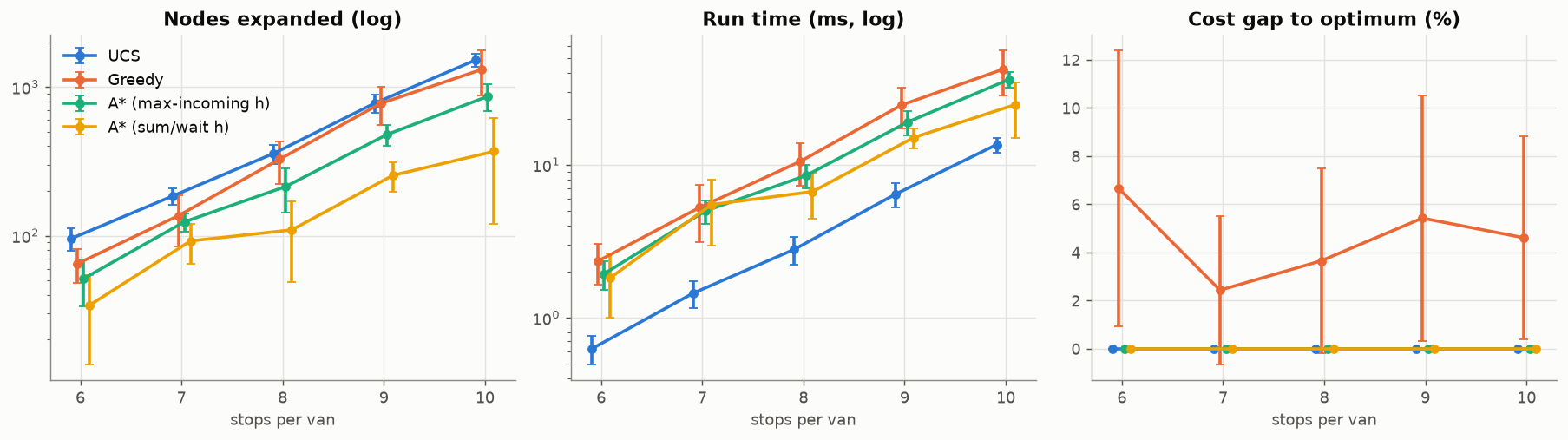
The obvious heuristic, "cheapest incoming trip at the current hour", is not admissible when travel times change through the day (our counter-example: 40 > 35). Our fix takes the minimum over all later departure times and adds a waiting bound. Step through the real A* trace for van 0 on the demo day:

Expansion 1

g, minutes so farh, admissible estimate left

f = g + h stays at 461 while h hands its estimate over to g. The bound is tight from the start because the time windows force most of the waiting.

Stops	Algorithm	Nodes expanded	Gap to optimum
6	UCS	95.5 ± 16.5	0%
6	Greedy	64.7 ± 16.4	6.7%
6	A*	34.0 ± 20.4	0%
10	UCS	1,519 ± 161	0%
10	Greedy	1,312 ± 440	4.6%
10	A*	368.7 ± 249	0%

10 seeds per size. A* matched brute force in 30/30 checks. At this size UCS is still faster in milliseconds, because each A* node costs more to evaluate.

Nodes expanded, cost gap and time for UCS, Greedy and A* from 6 to 10 stops — Experiment 1: A* vs UCS vs Greedy, 6 to 10 stops.

6Models line · stop 6 in the dossier

Van assignment

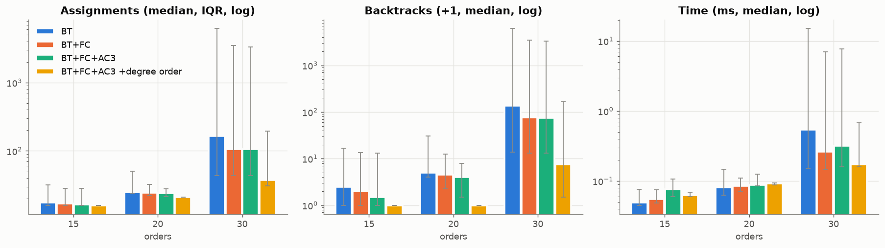
The same hard rush-hour instance (20 orders, windows 09:00 to 12:00, zero spare capacity, 4 rules from the NN), solved four ways. Pick a solver:

Bars show assignments tried. With only 3 values per variable and "≠" constraints AC-3 adds little; forward checking's capacity pruning and most-constrained-first ordering do most of the work.

Orders	Solver	Median assignments	Solved / unsat / limit
30	BT	165.5	8 / 0 / 2
30	BT + FC	105.5	8 / 0 / 2
30	BT + FC + AC-3	104.5	8 / 1 / 1
30	+ most-constrained first	36.5	9 / 1 / 0

CSP assignments and backtracks for 15, 20 and 30 orders — Experiment 2: BT vs FC vs AC-3 for 15, 20, 30 orders.

7System line · stop 7 in the dossier

Demo day

=== INTEGRATION LOOP (NN -> CSP -> A*) loop 1: CSP solved (rules: 2 from NN, 0 learned; 20 assignments, 0 backtracks) van 0 late by 2.1 min -> new rule: orders 16 and 5 on different vans loop 2: CSP solved (rules: 2 from NN, 1 learned; 20 assignments, 0 backtracks) status: ok -- all 20 orders on time after 2 loop(s)

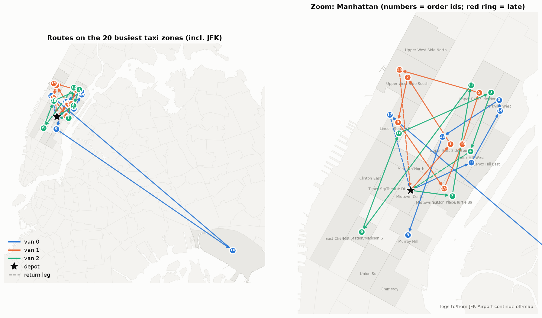
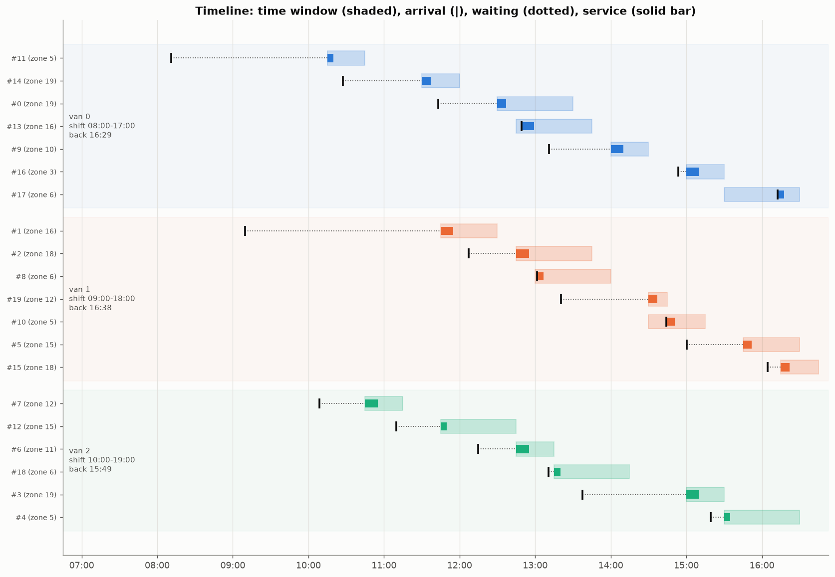
In loop 1, van 0 would serve JFK Airport (15:00–15:30) and then Upper East Side North (window from 15:45): 2.1 minutes late. That pair becomes a rule; in loop 2 every order is on time.

Map of the three van routes across Manhattan and JFK — Routes per van, with a zoom on Manhattan.

Timeline of each van showing time windows, arrivals, waiting and service — Timeline: window, arrival, waiting and service for every stop.

When there is no solution

Run with --impossible: order 0 moves to JFK with a window of 08:00–08:20.

NO SOLUTION: not every order can be served on time. Unserviceable orders / reasons: - order 0: window not reachable from the depot by any van: van 0: earliest arrival 08:48 is after the window closes 08:20 van 1: earliest arrival 09:46 is after the window closes 08:20 van 2: earliest arrival 10:43 is after the window closes 08:20 Suggestion: widening the windows of orders [0] by 30 min (15-min steps) makes it feasible.

10Evaluation line · stop 10 in the dossier

Replay with real trip times

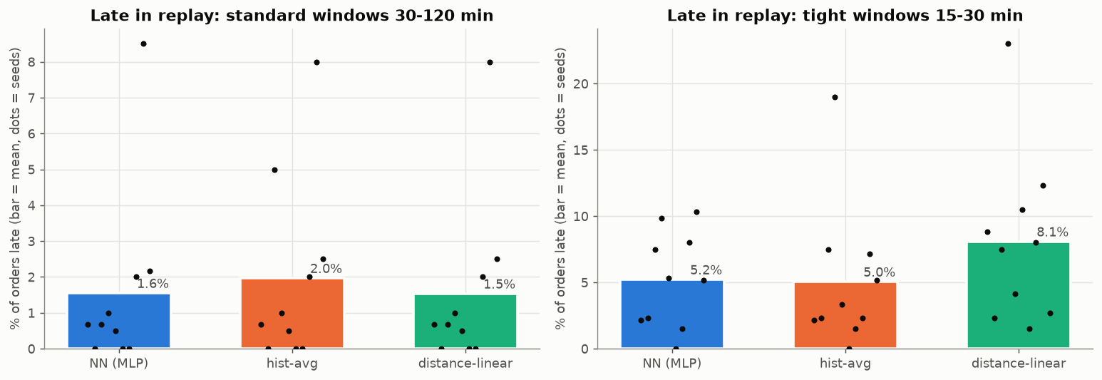
Each plan is replayed with real trip durations drawn from the held-out week, and late deliveries are counted. Experiment 3, 10 seeds per scenario:

With tight windows, hour-aware travel times (NN or historical) are late about 5% of the time versus 8% for distance only. With loose windows all three models are close, so the extra modelling only pays when the schedule is tight.

Late deliveries per model and scenario in the replay — Experiment 3: lateness in the replay.

Limits

Taxis are not vans: the 1.2 factor is a documented assumption, not a measurement.
Plans use mean times with no safety buffer, so 1–8% of deliveries are still late in the replay.
One month of data; seasonality and weather are not modelled.

8System line · stop 8 in the dossier

Run it

Python 3.13, plain numpy (no PyTorch or scikit-learn). All randomness is seeded.

python -m venv .venv
.venv\Scripts\activate            # Linux/macOS: source .venv/bin/activate
pip install -r requirements.txt

python make_data.py               # download 1 month (38 MB) and preprocess
python train_nn.py                # ~15 s: train MLP, baselines, time matrices
python -m pytest -q               # 38 tests: normal, edge and impossible cases
python run_demo.py                # demo day + outputs/demo_report.html
python run_demo.py --impossible   # the "NO SOLUTION" case
python run_experiments.py         # 3 experiments x 10 seeds